1 billion row challenge in SQL and Oracle Database

On the 1st of January 2024, Gunnar Morling launched The One Billion Row Challenge, fitting for a great start to the new year. As the challenge states:

Your mission, should you decide to accept it, is deceptively simple: write a Java program for retrieving temperature measurement values from a text file and calculating the min, mean, and max temperature per weather station. There’s just one caveat: the file has 1,000,000,000 rows!

Not surprisingly, the challenge has become widely popular on the internet and spilled over to other languages and technologies, including Go, Python, Rust, .NET, C, and, to no surprise SQL as well, given that SQL does well when it comes to aggregations.

Generating the data
Accessing the data
Aggregating the data
Creating an external table
- The SQL producing the desired output
Bonus #1: does it scale
Bonus #2: what about internal data?
- Bonus #2.1: Will the CTAS scale just as well as the SELECT did?
Bonus #3: What if the data is indexed?
Bonus #4: Using ORACLE_LOADER with IO_OPTIONS (NODIRECTIO) and explicit fields definition
Bonus #5: Using Materialized Views and Query Rewrite
Bonus #6: Returning 10,000 weather stations instead of 413
- Generating the file
- Running the query
  - Returning 413 rows
  - Returning 10,000 rows
Results
What’s next?

UPDATE 2024-03-01: Bonus #6 shows the query performance between 413 stations and 10,000 stations.

UPDATE 2024-02-05: Bonus #5 has been added, showing the benefits of Materialized Views and Query Rewrite.

UPDATE 2024-02-02: Bonus #4 has been added, making it the fastest solution for the external table read. Thanks to Loïc Lefèvre for finding this solution!

Naturally, I’m intrigued by how Oracle Database fits into this challenge. Although I do not care so much about how fast Oracle Database can process the data compared to the Java implementations. Naturally, with Java one can tailor a program for the exact challenge, leveraging SIMD APIs, bit shifting and all the good stuff that will give you the best possible performance without caring about being a multi-user, general-purpose, ACID compliant system. So there is definitely some overhead that can be saved when writing the Java program. What caught my attention is something different. I think that the broader goal of the original challenge was to motivate people to educate themselves about the mechanisms and features available in modern Java:

The goal of the 1BRC challenge is to create the fastest implementation for this task, and while doing so, explore the benefits of modern Java and find out how far you can push this platform. So grab all your (virtual) threads, reach out to the Vector API and SIMD, optimize your GC, leverage AOT compilation, or pull any other trick you can think of.

I’m quite a fan of this approach, as too often, we tend to blindly believe some random blog post or tweet about some technology not being up to the task or being the single best solution, without doing any proper due diligence. Hence I will follow this approach and focus more on highlighting the different mechanisms that Oracle Database provides to fulfill the task of the challenge. So hence the following note:

Note: The numbers highlighted in this blog are not a benchmark and should not be interpreted as the best possible solution one can achieve. Chances are high that the numbers will vary in your setup!

Generating the data

I follow similar instructions as outlined here.

Clone the repository https://github.com/gunnarmorling/1brc locally and cd into it:

$ git clone https://github.com/gunnarmorling/1brc.git
$ cd 1brc

Make sure you have Java 21 installed:

$ yum install openjdk@21

Build the data generator (I have it from good sources, aka Andres Almiray that clean is not needed when using verify):

$ ./mvnw verify

Generate the measurements file with 1 billion rows:

./create_measurements.sh 1000000000

The last step will run for a while (about 6 mins on my old Intel Mac) and spit out a 13GB text file:

$ ls -alh measurements.txt
-rw-r--r--. 1 oracle oinstall 13G Jan 13 02:50 measurements.txt
$ head measurements.txt
Tehran;16.9
Luanda;34.5
Columbus;0.3
Taipei;10.3
Djibouti;25.5
Kinshasa;21.4
Bosaso;20.8
Mexico City;2.3
Suva;39.5
Dushanbe;28.0

Accessing the data

For a long time, Oracle Database has offered the mechanism known as “External Table” to create a table inside Oracle DB that points to an external source, such as the generated measurements.txt file. This way, Oracle SQL can be run on external files just as if the data were residing in the database itself. To create such an external table, we first need a directory object inside the database that points to the external file and grant READ access to the user. This can be done (as a privileged user such as SYSTEM) with the following syntax:

SQL> CREATE DIRECTORY brc AS '/opt/oracle/1brc';

Directory created.

SQL> GRANT READ, WRITE ON DIRECTORY brc TO brc;

Grant succeeded.

Once the directory exists, an inline external table can be used by the user to query the data:

SQL> SELECT *
 FROM EXTERNAL
 (
   (
     station_name  VARCHAR2(26),
     measurement   NUMBER(3,1)
   )
   TYPE oracle_loader
   DEFAULT DIRECTORY brc
   ACCESS PARAMETERS
   (
     RECORDS DELIMITED BY NEWLINE
     FIELDS CSV WITHOUT EMBEDDED TERMINATED BY ';'
   )
   LOCATION ('measurements.txt')
   REJECT LIMIT UNLIMITED
 ) measurements
FETCH FIRST 10 ROWS ONLY;

STATION_NAME  MEASUREMENT
------------- -----------
Tehran               16.9
Luanda               34.5
Columbus               .3
Taipei               10.3
Djibouti             25.5
Kinshasa             21.4
Bosaso               20.8
Mexico City           2.3
Suva                 39.5
Dushanbe               28

10 rows selected.

This is quite a cool mechanism as it allows you to run Oracle SQL over external data directly, no need to load it if you don’t want to hold on to the data. One thing to remember, however, is that the access to the data is serial by default, as there is no parallel clause defined. Naturally, scanning 13GB of data serially will take longer than when accessing the data in parallel. This is quickly demonstrated when running something like a COUNT(*) over the external table:

SQL> set timing on;
SQL> SELECT COUNT(*)
  FROM EXTERNAL
  (
    (
      station_name  VARCHAR2(26),
      measurement   NUMBER(3,1)
    )
    TYPE oracle_loader
    DEFAULT DIRECTORY brc
    ACCESS PARAMETERS
    (
      RECORDS DELIMITED BY NEWLINE
      FIELDS CSV WITHOUT EMBEDDED TERMINATED BY ';'
    )
    LOCATION ('measurements.txt')
    REJECT LIMIT UNLIMITED
  ) measurements;

  COUNT(*)
----------
1000000000

Elapsed: 00:03:35.92

Instead, one can instruct the database via a hint to run in parallel, either by explicitly defining the parallelization level with /*+ PARALLEL (<number of parallel workers>) */, or by letting the database decide for itself how many parallel workers to use via just /*+ PARALLEL */. The important part here is the WITHOUT EMBEDDED in the external table definition above. As the Oracle Utilities documentation states:

The following are key points regarding the FIELDS CSV clause:

The default is to not use the FIELDS CSV clause.

The WITH EMBEDDED and WITHOUT EMBEDDED options specify whether record terminators are included (embedded) in the data. The WITH EMBEDDED option is the default.

If WITH EMBEDDED is used, then embedded record terminators must be enclosed, and intra-datafile parallelism is disabled for external table loads.

The TERMINATED BY ',' and OPTIONALLY ENCLOSED BY '"' options are the defaults and do not have to be specified. You can override them with different termination and enclosure characters.

So, to read a file in parallel, the external table definition requires WITHOUT EMBEDDED to be specified. Let’s see how much faster reading the file gets when running in parallel with 32 cores. 32 cores is the number of cores that compares to the server used to evaluate the Java programs competing in the challenge, so it seems adequate to use the similar parallelization level. However, note that the CPU model itself is different, so again, do not take these numbers as anything else but a comparison between running on a single core or 32 cores.

UPDATE: As it turns out, the server that is used to evaluate the Java programs comes with 32 cores with SMT enabled, raising the overall core count seen by the OS to 64, while the query below is only using half of that.

SQL> SELECT /*+ PARALLEL (32) */ COUNT(*)
  FROM EXTERNAL
  (
    (
      station_name  VARCHAR2(26),
      measurement   NUMBER(3,1)
    )
    TYPE oracle_loader
    DEFAULT DIRECTORY brc
    ACCESS PARAMETERS
    (
      RECORDS DELIMITED BY NEWLINE
      FIELDS CSV WITHOUT EMBEDDED TERMINATED BY ';'
    )
    LOCATION ('measurements.txt')
    REJECT LIMIT UNLIMITED
  ) measurements;

  COUNT(*)
----------
1000000000

Elapsed: 00:00:27.27

That’s much better, parallelization cut the time down significantly from the previous 3min 36 sec to just about 27 seconds. However, is there any other method of reading this file that could be even faster? Well, actually, there is! Oracle also provides other access parameters, or Access Drivers, for external tables. One of them is known as ORACLE_BIGDATA, introduced at a time when Big Data was still a thing (remember, about a decade ago, those were the days… not). The ORACLE_BIGDATA access driver can also read text files and parallelize them, the usage of it via an external table is pretty much the same. All that needs to change is the TYPE and the ACCESS PARAMETERS:

SQL> SELECT /*+ PARALLEL(32) */ COUNT(*)
  FROM EXTERNAL
  (
    (
      station_name  VARCHAR2(26),
      measurement   NUMBER(3,1)
    )
    TYPE oracle_bigdata
    DEFAULT DIRECTORY brc
    ACCESS PARAMETERS
    (
      com.oracle.bigdata.fileformat=csv
      com.oracle.bigdata.csv.rowformat.separatorcharacter=';'
    )
    LOCATION ('measurements.txt')
    REJECT LIMIT UNLIMITED
  ) measurements;

  COUNT(*)
----------
1000000000

Elapsed: 00:00:02.13

Wow, that is amazing, using the ORACLE_BIGDATA access driver, the database can now read the 13GB file in about 2 seconds when using 32 parallel workers. That’s quite a difference from the original 3 minutes and 36 seconds. 2 seconds seems to be good enough to move on to the next part of the challenge, aggregating the data and producing the desired result.

Aggregating the data

The challenge is not about reading 13GB of data as fast as possible, it is about calculating the min, average, and max temperature value per weather station. In the SQL world, such an aggregation can be easily accomplished via a GROUP BY like this:

SQL> SELECT /*+ PARALLEL (32) */
       station_name,
       MIN(measurement),
       AVG(measurement),
       MAX(measurement)
 FROM  EXTERNAL
  (
    (
      station_name  VARCHAR2(26),
      measurement   NUMBER(3,1)
    )
    TYPE oracle_bigdata
    DEFAULT DIRECTORY brc
    ACCESS PARAMETERS
    (
      com.oracle.bigdata.fileformat=csv
      com.oracle.bigdata.csv.rowformat.separatorcharacter=';'
    )
    LOCATION ('measurements.txt')
    REJECT LIMIT UNLIMITED
  ) measurements
  GROUP BY station_name;

STATION_NAME               MIN(MEASUREMENT) AVG(MEASUREMENT) MAX(MEASUREMENT)
-------------------------- ---------------- ---------------- ----------------
Nouakchott                            -21.5       25.7011478             73.1
Alexandria                            -30.4       19.9867241             70.9
Pretoria                              -30.6        18.184254             66.1
Oulu                                  -52.6       2.69914531             52.3
Abha                                  -33.6        18.000858             65.1
San Juan                              -22.8       27.2043868             75.8
...
...
...
Nairobi                               -41.7       17.7956014             65.8
Chiang Mai                            -25.6       25.8109352             77.4
San Jose                              -31.7       22.6019843             70.4
Garissa                               -23.3       29.2899336             78.3

413 rows selected.

Elapsed: 00:00:08.18

As you can see above, the overall execution time increased from 2 seconds just reading the data to 8 seconds also performing the calculation. The result, however, is not yet complete. The challenge states the following conditions:

sorted alphabetically by station name
the result values per station in the format <min>/<mean>/<max>
rounded to one fractional digit
results emitted in a format like this: {Abha=-23.0/18.0/59.2, Abidjan=-16.2/26.0/67.3, …}

To achieve the above stated challenge conditions, we need to do a couple of more things. The average/mean temperature needs to be rounded to one fraction, and the result needs to be in one long, sorted string, instead of 413 rows returned. For that, we need to do a bit more SQL magic. But before we get to that, I want to show another little trick first.

Creating an external table

The above SQL statement has already gotten quite a bit lengthy due to the inline external table definition. However, there is a reason why it’s called an “External Table”. Oracle Database allows you to store the definition of the access parameters as a table and then query it as if it were any other (internal) table. All you have to do is to wrap the EXTERNAL() parameters into a CREATE TABLE statement:

SQL> CREATE TABLE measurements_ext
(
  station_name  VARCHAR2(26),
  measurement   NUMBER(3,1)
)
ORGANIZATION EXTERNAL
(
  TYPE oracle_bigdata
  DEFAULT DIRECTORY brc
  ACCESS PARAMETERS
  (
    com.oracle.bigdata.fileformat=csv
    com.oracle.bigdata.csv.rowformat.separatorcharacter=';'
  )
  LOCATION ('measurements.txt')
)
REJECT LIMIT UNLIMITED;

Table created.

And from now on, the the file can be queried as if it were any other table in the database:

SQL> desc measurements_ext
 Name         Null? Type
 ------------ ----- ------------
 STATION_NAME       VARCHAR2(26)
 MEASUREMENT        NUMBER(3,1)

SQL> SELECT /*+ PARALLEL (32) */ COUNT(*) FROM measurements_ext;

  COUNT(*)
----------
1000000000

Elapsed: 00:00:02.03

Note that I’ve called the table measurements_ext to make it clear that it is an external table.

The SQL producing the desired output

With the external table in place, we can shorten our SQL statement FROM clause just down to the table and complete it to fulfill the challenge requirements:

SELECT '{' ||
          LISTAGG(station_name || '=' || min_measurement || '/' || mean_measurement || '/' || max_measurement, ', ')
            WITHIN GROUP (ORDER BY station_name) ||
       '}' AS "1BRC"
 FROM
  (SELECT station_name,
          MIN(measurement) AS min_measurement,
          ROUND(AVG(measurement), 1) AS mean_measurement,
          MAX(measurement) AS max_measurement
    FROM measurements_ext
     GROUP BY station_name
  );

What has happened here? At a closer look, you will see that the aggregation now occurs in a sub-select in the FROM clause. It’s the same aggregation as before, with the one exception that we now use the ROUND function over the AVG function to round the mean temperature to one fraction. Based on that result from the sub-select, we use the LISTAGG function to pivot the output rows into one long list in the desired format. Note the ORDER BY station_name that will guarantee that the list is in order. Last but not least, we wrap around the opening and closing curly braces.

When running (in parallel) again, we get the following timing:

SQL> SELECT /*+ PARALLEL (32) */
       '{' ||
          LISTAGG(station_name || '=' || min_measurement || '/' || mean_measurement || '/' || max_measurement, ', ')
            WITHIN GROUP (ORDER BY station_name) ||
       '}' AS "1BRC"
 FROM
  (SELECT station_name,
          MIN(measurement) AS min_measurement,
          ROUND(AVG(measurement), 1) AS mean_measurement,
          MAX(measurement) AS max_measurement
    FROM measurements_ext
     GROUP BY station_name
  );

1BRC
--------------------------------------------------------------------------------
{Abha=-33.6/18/65.1, Abidjan=-25.4/26/73.9, Abéché=-21.1/29.4/79.7, Accra=-23.2/
26.4/76.9, Addis Ababa=-36.5/16/68.9, Adelaide=-29.7/17.3/66.4, Aden=-18.8/29.1/
81.5, Ahvaz=-25.1/25.4/78.1, Albuquerque=-39.7/14/65.2, Alexandra=-38.4/11/61.3,
 Alexandria=-30.4/20/70.9, Algiers=-32.3/18.2/70.8, Alice Springs=-28.3/21/71,
...
...
...
Whitehorse=-50.6/-.1/52, Wichita=-40.3/13.9/65.8, Willemstad=-23.4/28/74.3, Winn
ipeg=-46/3/58.4, Wrocław=-42.1/9.6/57.3, Xi'an=-33.9/14.1/65.6, Yakutsk=-64.5/-8
.8/41.2, Yangon=-22/27.5/75.9, Yaoundé=-26.1/23.8/72, Yellowknife=-54.5/-4.3/48.
2, Yerevan=-35.9/12.4/62.9, Yinchuan=-39.1/9/61.9, Zagreb=-38.4/10.7/60.8, Zanzi
bar City=-26.8/26/76.2, Zürich=-42.7/9.3/62.8, Ürümqi=-39.9/7.4/56.1, İzmir=-36.
3/17.9/68.8}

Elapsed: 00:00:08.12

Note that the execution time of this single-row generating query is not different from returning the 413 rows before, meaning that producing the desired output does not add significant overhead to the overall execution.

So, there you have it, Oracle Database can produce the same result using SQL over an external file, parallelized, in about 8 seconds. No knowledge of SIMD APIs or bit shifting or anything else is required, just SQL, the concept of (inline) external tables, and the ORACLE_BIGDATA access drivers. Furthermore, this demonstrates that not only can Oracle Database perform SQL on external data, but also that 1 billion rows in a table is nothing to be concerned with, Oracle Database can handle it just fine.

Bonus #1: does it scale

Some of you may ask yourself now, “But what if I have more than 32 cores? Does it scale?” Well, I happen to have more cores on the machine available, 128 to be precise, so let’s see how this would look like with 64 cores:

SQL> SELECT /*+ PARALLEL (64) */
       '{' ||
          LISTAGG(station_name || '=' || min_measurement || '/' || mean_measurement || '/' || max_measurement, ', ')
            WITHIN GROUP (ORDER BY station_name) ||
       '}' AS "1BRC"
 FROM
  (SELECT station_name,
          MIN(measurement) AS min_measurement,
          ROUND(AVG(measurement), 1) AS mean_measurement,
          MAX(measurement) AS max_measurement
    FROM measurements_ext
     GROUP BY station_name
  );

1BRC
--------------------------------------------------------------------------------
{Abha=-33.6/18/65.1, Abidjan=-25.4/26/73.9, Abéché=-21.1/29.4/79.7, Accra=-23.2/
26.4/76.9, Addis Ababa=-36.5/16/68.9, Adelaide=-29.7/17.3/66.4, Aden=-18.8/29.1/
81.5, Ahvaz=-25.1/25.4/78.1, Albuquerque=-39.7/14/65.2, Alexandra=-38.4/11/61.3,
 Alexandria=-30.4/20/70.9, Algiers=-32.3/18.2/70.8, Alice Springs=-28.3/21/71,
...
...
...
Whitehorse=-50.6/-.1/52, Wichita=-40.3/13.9/65.8, Willemstad=-23.4/28/74.3, Winn
ipeg=-46/3/58.4, Wrocław=-42.1/9.6/57.3, Xi'an=-33.9/14.1/65.6, Yakutsk=-64.5/-8
.8/41.2, Yangon=-22/27.5/75.9, Yaoundé=-26.1/23.8/72, Yellowknife=-54.5/-4.3/48.
2, Yerevan=-35.9/12.4/62.9, Yinchuan=-39.1/9/61.9, Zagreb=-38.4/10.7/60.8, Zanzi
bar City=-26.8/26/76.2, Zürich=-42.7/9.3/62.8, Ürümqi=-39.9/7.4/56.1, İzmir=-36.
3/17.9/68.8}

Elapsed: 00:00:04.61

Twice the core power (32 –> 64) equals half the execution time (8s –> 4s), so this scales very well. Ok, what about all 128 cores? We have to know now, right?

SQL> SELECT /*+ PARALLEL (128) */
       '{' ||
          LISTAGG(station_name || '=' || min_measurement || '/' || mean_measurement || '/' || max_measurement, ', ')
            WITHIN GROUP (ORDER BY station_name) ||
       '}' AS "1BRC"
 FROM
  (SELECT station_name,
          MIN(measurement) AS min_measurement,
          ROUND(AVG(measurement), 1) AS mean_measurement,
          MAX(measurement) AS max_measurement
    FROM measurements_ext
     GROUP BY station_name
  );

1BRC
--------------------------------------------------------------------------------
{Abha=-33.6/18/65.1, Abidjan=-25.4/26/73.9, Abéché=-21.1/29.4/79.7, Accra=-23.2/
26.4/76.9, Addis Ababa=-36.5/16/68.9, Adelaide=-29.7/17.3/66.4, Aden=-18.8/29.1/
81.5, Ahvaz=-25.1/25.4/78.1, Albuquerque=-39.7/14/65.2, Alexandra=-38.4/11/61.3,
 Alexandria=-30.4/20/70.9, Algiers=-32.3/18.2/70.8, Alice Springs=-28.3/21/71,
...
...
...
Whitehorse=-50.6/-.1/52, Wichita=-40.3/13.9/65.8, Willemstad=-23.4/28/74.3, Winn
ipeg=-46/3/58.4, Wrocław=-42.1/9.6/57.3, Xi'an=-33.9/14.1/65.6, Yakutsk=-64.5/-8
.8/41.2, Yangon=-22/27.5/75.9, Yaoundé=-26.1/23.8/72, Yellowknife=-54.5/-4.3/48.
2, Yerevan=-35.9/12.4/62.9, Yinchuan=-39.1/9/61.9, Zagreb=-38.4/10.7/60.8, Zanzi
bar City=-26.8/26/76.2, Zürich=-42.7/9.3/62.8, Ürümqi=-39.9/7.4/56.1, İzmir=-36.
3/17.9/68.8}

Elapsed: 00:00:04.05

No significant improvement can be seen. Yes, we saved about half a second of execution time, but with double the CPU power, suggesting that we have hit the ceiling somewhere between 64 and 128 cores.

Bonus #2: what about internal data?

Up until now, every time we executed the SQL statement, we told the Oracle Database to open and read a CSV file. However, it’s probably fair to say that if someone has a database, the data would be loaded once into a table and then queries many times (and in different ways) from there. So, let’s load the data into the database and see how the query behaves when the data resides inside an Oracle Database. Before, I called the external table measurements_ext so that we can clearly distinguish between the external table, aka CSV file and internal tables. This comes in handy now, as loading the data into the database is fairly straight forward now. All one has to do is to run a CREATE TABLE AS SELECT statement, commonly referred to as CTAS.

Just like before, also creating the table can run in parallel by specifying the PARALLEL clause. Furthermore, the NOLOGGING clause can be specified that instructs the database not to generate and write any redo information into the REDO logs. This is often an additional performance booster on busy systems where active users also generate plenty of redo. However, in this case it should not matter much as the system is otherwise idle and the disk is not a bottleneck. For good measure, I’ll demonstrate the usage of both.

Without NOLOGGING:

SQL> CREATE TABLE measurements
PARALLEL 32
AS SELECT * FROM measurements_ext;

Table created.

Elapsed: 00:02:03.16

With NOLOGGING:

SQL> drop table measurements;

Table dropped.

Elapsed: 00:00:00.05
SQL> purge user_recyclebin;

Recyclebin purged.

Elapsed: 00:00:00.02
SQL> CREATE TABLE measurements
PARALLEL 32
NOLOGGING
AS SELECT * FROM measurements_ext;
 
Table created.

Elapsed: 00:02:09.21

As you can see, there is no significant difference between the two. And, as it turns out, loading the data into the database is quite a bit more involved than just reading the data from an external file. This is an interesting observation to keep in mind. If you do not need the data to be in the database but just want to run a quick query over it and move on, you might be faster going the external table route.

Ok, next question, will the CREATE TABLE scale just as well as the SELECT did?

Bonus #2.1: Will the CTAS scale just as well as the SELECT did?

What happens if we use the same 64 cores as before? Will the table creation time be cut in half?

SQL> drop table measurements;

Table dropped.

Elapsed: 00:00:00.01
SQL> purge user_recyclebin;

Recyclebin purged.

Elapsed: 00:00:00.02
SQL> CREATE TABLE measurements
PARALLEL 64
AS SELECT * FROM measurements_ext;

Table created.

Elapsed: 00:01:56.24

The answer is, unfortunately, not, but we do save a little bit, an additional 13 seconds that is.

Ok, now that the data is in the database, how do the queries compare to before? Let’s start with the COUNT(*):

SQL> SELECT /*+ PARALLEL (32) */ COUNT(*) FROM measurements;

  COUNT(*)
----------
1000000000

Elapsed: 00:00:00.45

Ok wow, that’s gotten super fast, less than a second. How about the actual query (note the FROM clause now refers to measurements instead of previously measurements_ext):

SQL> SELECT /*+ PARALLEL (32) */
       '{' ||
          LISTAGG(station_name || '=' || min_measurement || '/' || mean_measurement || '/' || max_measurement, ', ')
            WITHIN GROUP (ORDER BY station_name) ||
       '}' AS "1BRC"
 FROM
  (SELECT station_name,
          MIN(measurement) AS min_measurement,
          ROUND(AVG(measurement), 1) AS mean_measurement,
          MAX(measurement) AS max_measurement
    FROM measurements
     GROUP BY station_name
  );

1BRC
--------------------------------------------------------------------------------
{Abha=-33.6/18/65.1, Abidjan=-25.4/26/73.9, Abéché=-21.1/29.4/79.7, Accra=-23.2/
26.4/76.9, Addis Ababa=-36.5/16/68.9, Adelaide=-29.7/17.3/66.4, Aden=-18.8/29.1/
81.5, Ahvaz=-25.1/25.4/78.1, Albuquerque=-39.7/14/65.2, Alexandra=-38.4/11/61.3,
 Alexandria=-30.4/20/70.9, Algiers=-32.3/18.2/70.8, Alice Springs=-28.3/21/71,
...
...
...
Whitehorse=-50.6/-.1/52, Wichita=-40.3/13.9/65.8, Willemstad=-23.4/28/74.3, Winn
ipeg=-46/3/58.4, Wrocław=-42.1/9.6/57.3, Xi'an=-33.9/14.1/65.6, Yakutsk=-64.5/-8
.8/41.2, Yangon=-22/27.5/75.9, Yaoundé=-26.1/23.8/72, Yellowknife=-54.5/-4.3/48.
2, Yerevan=-35.9/12.4/62.9, Yinchuan=-39.1/9/61.9, Zagreb=-38.4/10.7/60.8, Zanzi
bar City=-26.8/26/76.2, Zürich=-42.7/9.3/62.8, Ürümqi=-39.9/7.4/56.1, İzmir=-36.
3/17.9/68.8}

Elapsed: 00:00:04.02

Also, the resulting query is twice as fast as before, 4 seconds instead of the previous 8 seconds! Next, the usual question: Does it scale? What about 64 cores?

SQL> SELECT /*+ PARALLEL (64) */
       '{' ||
          LISTAGG(station_name || '=' || min_measurement || '/' || mean_measurement || '/' || max_measurement, ', ')
            WITHIN GROUP (ORDER BY station_name) ||
       '}' AS "1BRC"
 FROM
  (SELECT station_name,
          MIN(measurement) AS min_measurement,
          ROUND(AVG(measurement), 1) AS mean_measurement,
          MAX(measurement) AS max_measurement
    FROM measurements
     GROUP BY station_name
  );

1BRC
--------------------------------------------------------------------------------
{Abha=-33.6/18/65.1, Abidjan=-25.4/26/73.9, Abéché=-21.1/29.4/79.7, Accra=-23.2/
26.4/76.9, Addis Ababa=-36.5/16/68.9, Adelaide=-29.7/17.3/66.4, Aden=-18.8/29.1/
81.5, Ahvaz=-25.1/25.4/78.1, Albuquerque=-39.7/14/65.2, Alexandra=-38.4/11/61.3,
 Alexandria=-30.4/20/70.9, Algiers=-32.3/18.2/70.8, Alice Springs=-28.3/21/71,
...
...
...
Whitehorse=-50.6/-.1/52, Wichita=-40.3/13.9/65.8, Willemstad=-23.4/28/74.3, Winn
ipeg=-46/3/58.4, Wrocław=-42.1/9.6/57.3, Xi'an=-33.9/14.1/65.6, Yakutsk=-64.5/-8
.8/41.2, Yangon=-22/27.5/75.9, Yaoundé=-26.1/23.8/72, Yellowknife=-54.5/-4.3/48.
2, Yerevan=-35.9/12.4/62.9, Yinchuan=-39.1/9/61.9, Zagreb=-38.4/10.7/60.8, Zanzi
bar City=-26.8/26/76.2, Zürich=-42.7/9.3/62.8, Ürümqi=-39.9/7.4/56.1, İzmir=-36.
3/17.9/68.8}

Elapsed: 00:00:02.28

And the answer is: Oh yes, it does. We are down to 2 seconds! That’s twice as fast as reading the data from the external file! What about 128 cores, i.e. all the CPU power we got:

SQL> SELECT /*+ PARALLEL (128) */
       '{' ||
          LISTAGG(station_name || '=' || min_measurement || '/' || mean_measurement || '/' || max_measurement, ', ')
            WITHIN GROUP (ORDER BY station_name) ||
       '}' AS "1BRC"
 FROM
  (SELECT station_name,
          MIN(measurement) AS min_measurement,
          ROUND(AVG(measurement), 1) AS mean_measurement,
          MAX(measurement) AS max_measurement
    FROM measurements
     GROUP BY station_name
  );

1BRC
--------------------------------------------------------------------------------
{Abha=-33.6/18/65.1, Abidjan=-25.4/26/73.9, Abéché=-21.1/29.4/79.7, Accra=-23.2/
26.4/76.9, Addis Ababa=-36.5/16/68.9, Adelaide=-29.7/17.3/66.4, Aden=-18.8/29.1/
81.5, Ahvaz=-25.1/25.4/78.1, Albuquerque=-39.7/14/65.2, Alexandra=-38.4/11/61.3,
 Alexandria=-30.4/20/70.9, Algiers=-32.3/18.2/70.8, Alice Springs=-28.3/21/71,
...
...
...
Whitehorse=-50.6/-.1/52, Wichita=-40.3/13.9/65.8, Willemstad=-23.4/28/74.3, Winn
ipeg=-46/3/58.4, Wrocław=-42.1/9.6/57.3, Xi'an=-33.9/14.1/65.6, Yakutsk=-64.5/-8
.8/41.2, Yangon=-22/27.5/75.9, Yaoundé=-26.1/23.8/72, Yellowknife=-54.5/-4.3/48.
2, Yerevan=-35.9/12.4/62.9, Yinchuan=-39.1/9/61.9, Zagreb=-38.4/10.7/60.8, Zanzi
bar City=-26.8/26/76.2, Zürich=-42.7/9.3/62.8, Ürümqi=-39.9/7.4/56.1, İzmir=-36.
3/17.9/68.8}

Elapsed: 00:00:01.85

Using all the cores, we just about manage to get the processing time below 2 seconds, so it seems that about 2 seconds is as good as it gets. That is still very impressive if you think about it. Oracle Database manages to scan and aggregate 1 billion rows in about 4 seconds on this particular 32-core machine, which is certainly not far behind the fasted Java implementations that were submitted to the challenge. The perhaps most important takeaway here is that Oracle Database (and SQL) can definitely keep up with modern programming languages!

Bonus #3: What if the data is indexed?

Typically, data residing in a database usually has some indexes on it. That allows the database for faster access methods and further optimization. So, let’s see whether there would be any additional benefit if both columns for the table would also be indexed:

SQL> CREATE INDEX measurements_idx_001
 ON measurements(station_name, measurement)
 PARALLEL 32;

Index created.

Elapsed: 00:02:31.90
SQL> -- Gather schema (including index) stats
SQL> exec dbms_stats.gather_schema_stats(ownname=>user, estimate_percent=>null, cascade=>true, degree=>64);

PL/SQL procedure successfully completed.

Elapsed: 00:00:38.99
SQL> SELECT /*+ PARALLEL (32) */
       '{' ||
          LISTAGG(station_name || '=' || min_measurement || '/' || mean_measurement || '/' || max_measurement, ', ')
            WITHIN GROUP (ORDER BY station_name) ||
       '}' AS "1BRC"
 FROM
  (SELECT station_name,
          MIN(measurement) AS min_measurement,
          ROUND(AVG(measurement), 1) AS mean_measurement,
          MAX(measurement) AS max_measurement
    FROM measurements
     GROUP BY station_name
  );

1BRC
--------------------------------------------------------------------------------
{Abha=-33.6/18/65.1, Abidjan=-25.4/26/73.9, Abeche=-21.1/29.4/79.7, Accra=-23.2/
26.4/76.9, Addis Ababa=-36.5/16/68.9, Adelaide=-29.7/17.3/66.4, Aden=-18.8/29.1/
81.5, Ahvaz=-25.1/25.4/78.1, Albuquerque=-39.7/14/65.2, Alexandra=-38.4/11/61.3,
 Alexandria=-30.4/20/70.9, Algiers=-32.3/18.2/70.8, Alice Springs=-28.3/21/71,
...
...
...
Whitehorse=-50.6/-.1/52, Wichita=-40.3/13.9/65.8, Willemstad=-23.4/28/74.3, Winn
ipeg=-46/3/58.4, Wroclaw=-42.1/9.6/57.3, Xi'an=-33.9/14.1/65.6, Yakutsk=-64.5/-8
.8/41.2, Yangon=-22/27.5/75.9, Yaounde=-26.1/23.8/72, Yellowknife=-54.5/-4.3/48.
2, Yerevan=-35.9/12.4/62.9, Yinchuan=-39.1/9/61.9, Zagreb=-38.4/10.7/60.8, Zanzi
bar City=-26.8/26/76.2, Zurich=-42.7/9.3/62.8, Urumqi=-39.9/7.4/56.1, ?zmir=-36.
3/17.9/68.8}

Elapsed: 00:00:03.84

Hm, although the overall execution time decreased slightly, having an index on the table columns doesn’t seem to make much of a difference. The easiest way to find out whether the index was used or not, is by retrieving the execution plan for the query. This can be done easiest via set autotrace on (although that requires SELECT privileges on certain v$ views, which is granted easiest via GRANT SELECT_CATALOG_ROLE TO <user>)

SQL> set autotrace on;
SQL> SELECT /*+ PARALLEL (32) */
       '{' ||
          LISTAGG(station_name || '=' || min_measurement || '/' || mean_measurement || '/' || max_measurement, ', ')
            WITHIN GROUP (ORDER BY station_name) ||
       '}' AS "1BRC"
 FROM
  (SELECT station_name,
          MIN(measurement) AS min_measurement,
          ROUND(AVG(measurement), 1) AS mean_measurement,
          MAX(measurement) AS max_measurement
    FROM measurements
     GROUP BY station_name
  );

1BRC
--------------------------------------------------------------------------------
{Abha=-33.6/18/65.1, Abidjan=-25.4/26/73.9, Abeche=-21.1/29.4/79.7, Accra=-23.2/
26.4/76.9, Addis Ababa=-36.5/16/68.9, Adelaide=-29.7/17.3/66.4, Aden=-18.8/29.1/
81.5, Ahvaz=-25.1/25.4/78.1, Albuquerque=-39.7/14/65.2, Alexandra=-38.4/11/61.3,
 Alexandria=-30.4/20/70.9, Algiers=-32.3/18.2/70.8, Alice Springs=-28.3/21/71,
...
...
...
Elapsed: 00:00:03.79

Execution Plan
----------------------------------------------------------
Plan hash value: 3606041051

------------------------------------------------------------------------------------------------------------------------
| Id  | Operation                  | Name         | Rows  | Bytes | Cost (%CPU)| Time     |    TQ  |IN-OUT| PQ Distrib |
------------------------------------------------------------------------------------------------------------------------
|   0 | SELECT STATEMENT           |              |     1 |    54 | 24838   (6)| 00:00:01 |        |      |            |
|   1 |  SORT GROUP BY             |              |     1 |    54 |            |          |        |      |            |
|   2 |   PX COORDINATOR           |              |       |       |            |          |        |      |            |
|   3 |    PX SEND QC (RANDOM)     | :TQ10001     |   413 | 22302 | 24838   (6)| 00:00:01 |  Q1,01 | P->S | QC (RAND)  |
|   4 |     VIEW                   |              |   413 | 22302 | 24838   (6)| 00:00:01 |  Q1,01 | PCWP |            |
|   5 |      HASH GROUP BY         |              |   413 |  5369 | 24838   (6)| 00:00:01 |  Q1,01 | PCWP |            |
|   6 |       PX RECEIVE           |              |   413 |  5369 | 24838   (6)| 00:00:01 |  Q1,01 | PCWP |            |
|   7 |        PX SEND HASH        | :TQ10000     |   413 |  5369 | 24838   (6)| 00:00:01 |  Q1,00 | P->P | HASH       |
|   8 |         HASH GROUP BY      |              |   413 |  5369 | 24838   (6)| 00:00:01 |  Q1,00 | PCWP |            |
|   9 |          PX BLOCK ITERATOR |              |  1000M|    12G| 23547   (1)| 00:00:01 |  Q1,00 | PCWC |            |
|  10 |           TABLE ACCESS FULL| MEASUREMENTS |  1000M|    12G| 23547   (1)| 00:00:01 |  Q1,00 | PCWP |            |
------------------------------------------------------------------------------------------------------------------------

Note
-----
   - Degree of Parallelism is 32 because of hint


Statistics
----------------------------------------------------------
        192  recursive calls
          0  db block gets
    2498416  consistent gets
          0  physical reads
          0  redo size
      10908  bytes sent via SQL*Net to client
        835  bytes received via SQL*Net from client
          2  SQL*Net roundtrips to/from client
          1  sorts (memory)
          0  sorts (disk)
          1  rows processed

And indeed, the plan shows that no index has been used by the query above, so we can strike that idea for that particular challenge. However, that doesn’t mean that an index wouldn’t be useful for other queries, for example, retrieving the measurements for a particular station:

SQL> SELECT '{' ||
          LISTAGG(station_name || '=' || min_measurement || '/' || mean_measurement || '/' || max_measurement, ', ')
            WITHIN GROUP (ORDER BY station_name) ||
       '}' AS "1BRC"
 FROM
  (SELECT station_name,
          MIN(measurement) AS min_measurement,
          ROUND(AVG(measurement), 1) AS mean_measurement,
          MAX(measurement) AS max_measurement
    FROM measurements
     WHERE station_name = 'Vienna'
     GROUP BY station_name
  );

1BRC
-------------------------------
{Vienna=-39.7/10.4/58.4}

Elapsed: 00:00:00.42

Execution Plan
-----------------------------------
Plan hash value: 2247006719

-----------------------------------------------------------------------------------------------
| Id  | Operation              | Name                 | Rows  | Bytes | Cost (%CPU)| Time     |
-----------------------------------------------------------------------------------------------
|   0 | SELECT STATEMENT       |                      |     1 |    44 |  8098   (1)| 00:00:01 |
|   1 |  SORT GROUP BY         |                      |     1 |    44 |            |          |
|   2 |   VIEW                 |                      |  2421K|   101M|  8098   (1)| 00:00:01 |
|   3 |    SORT GROUP BY NOSORT|                      |  2421K|    30M|  8098   (1)| 00:00:01 |
|*  4 |     INDEX RANGE SCAN   | MEASUREMENTS_IDX_001 |  2421K|    30M|  8098   (1)| 00:00:01 |
-----------------------------------------------------------------------------------------------

Predicate Information (identified by operation id):
---------------------------------------------------

   4 - access("STATION_NAME"='Vienna')


Statistics
----------------------------------------------------------
          1  recursive calls
          0  db block gets
       7438  consistent gets
          0  physical reads
          0  redo size
        568  bytes sent via SQL*Net to client
        842  bytes received via SQL*Net from client
          2  SQL*Net roundtrips to/from client
          1  sorts (memory)
          0  sorts (disk)
          1  rows processed

Note that the above query no longer runs in parallel, yet, thanks to the INDEX RANGE SCAN, the station and its measurements are retrieved in less than a second. Furthermore, the plan above shows no sign of the original table anymore. Because both columns the query requires are in the index, the table no longer needs to be accessed to retrieve any data. Instead, all information is retrieved from the index directly. That is even more impressive because there are over 2.4 million rows for that station alone:

SQL> SELECT COUNT(*) FROM measurements WHERE station_name = 'Vienna';

  COUNT(*)
----------
   2422649

Bonus #4: Using ORACLE_LOADER with IO_OPTIONS (NODIRECTIO) and explicit fields definition

My colleague and performance wizard Loïc Lefèvre took the time to read through the Performance Hints When Using the ORACLE_LOADER Access Driver section of the ORACLE_LOADER documentation and discovered further opportunities for performance improvement. Thanks, Loïc!

Oddly enough, Direct I/O is often used as a performance improvement mechanism, telling the OS not to spend any memory for caching the file but instead leaving it available for the programs. In this challenge, however, the fastest solution all map the file into memory, and so does the ORACLE_BIGDATA driver. So, it’s only fair to do the same with the ORACLE_LOADER driver. To recall, the original timing for the SELECT COUNT(*) with 32 parallel cores was about 27 seconds. Let’s see what the same query does with Direct I/O turned off:

SQL> set timing on;
SQL> SELECT /*+ PARALLEL (32) */ COUNT(*)
  FROM EXTERNAL
  (
    (
      station_name  VARCHAR2(26),
      measurement   NUMBER(3,1)
    )
    TYPE oracle_loader
    DEFAULT DIRECTORY brc
    ACCESS PARAMETERS
    (
      RECORDS DELIMITED BY NEWLINE
      IO_OPTIONS (NODIRECTIO)
      FIELDS CSV WITHOUT EMBEDDED TERMINATED BY ';'
    )
    LOCATION ('measurements.txt')
    REJECT LIMIT UNLIMITED
  ) measurements;

  COUNT(*)
----------
1000000000

Elapsed: 00:00:05.98

Now that is significantly faster than before and very close to the ORACLE_BIGDATA access driver. However, Loïc also discovered some additional benefits that aren’t explicitly stated in the section of the documentation. For example, not using FIELD CSV but an explicit definition further increased the performance:

SQL> SELECT /*+ PARALLEL (32) */ COUNT(*)
  FROM EXTERNAL
  (
    (
      station_name  VARCHAR2(26),
      measurement   NUMBER(3,1)
    )
    TYPE oracle_loader
    DEFAULT DIRECTORY brc
    ACCESS PARAMETERS
    (
      RECORDS DELIMITED BY NEWLINE
      IO_OPTIONS (NODIRECTIO)
      FIELDS TERMINATED BY ';'
      (
        station_name CHAR(26),
        measurement  CHAR(5)
      )
    )
    LOCATION ('measurements.txt')
    REJECT LIMIT UNLIMITED
  ) measurements;

  COUNT(*)
----------
1000000000

Elapsed: 00:00:03.62

And indeed, the query is now down to 3.6 seconds, which is almost as fast as the ORACLE_BIGDATA access driver with 2.1 seconds. Now, let’s see how this compares to the full query:

SQL> SELECT /*+ PARALLEL (32) */
       '{' ||
          LISTAGG(station_name || '=' || min_measurement || '/' || mean_measurement || '/' || max_measurement, ', ')
            WITHIN GROUP (ORDER BY station_name) ||
       '}' AS "1BRC"
 FROM
  (SELECT station_name,
          MIN(measurement) AS min_measurement,
          ROUND(AVG(measurement), 1) AS mean_measurement,
          MAX(measurement) AS max_measurement
   FROM EXTERNAL
   (
     (
       station_name  VARCHAR2(26),
       measurement   NUMBER(3,1)
     )
     TYPE oracle_loader
     DEFAULT DIRECTORY brc
     ACCESS PARAMETERS
     (
       RECORDS DELIMITED BY NEWLINE
       IO_OPTIONS (NODIRECTIO)
       FIELDS TERMINATED BY ';'
       (
         station_name  CHAR(26),
         measurement  CHAR(5)
       )
     )
     LOCATION ('measurements.txt')
     REJECT LIMIT UNLIMITED
   )
   GROUP BY station_name
  );

1BRC
--------------------------------------------------------------------------------
{Abha=-33.6/18/65.1, Abidjan=-25.4/26/73.9, Abéché=-21.1/29.4/79.7, Accra=-23.2/
26.4/76.9, Addis Ababa=-36.5/16/68.9, Adelaide=-29.7/17.3/66.4, Aden=-18.8/29.1/
81.5, Ahvaz=-25.1/25.4/78.1, Albuquerque=-39.7/14/65.2, Alexandra=-38.4/11/61.3,
 Alexandria=-30.4/20/70.9, Algiers=-32.3/18.2/70.8, Alice Springs=-28.3/21/71,
...
...
...
Whitehorse=-50.6/-.1/52, Wichita=-40.3/13.9/65.8, Willemstad=-23.4/28/74.3, Winn
ipeg=-46/3/58.4, Wrocław=-42.1/9.6/57.3, Xi'an=-33.9/14.1/65.6, Yakutsk=-64.5/-8
.8/41.2, Yangon=-22/27.5/75.9, Yaoundé=-26.1/23.8/72, Yellowknife=-54.5/-4.3/48.
2, Yerevan=-35.9/12.4/62.9, Yinchuan=-39.1/9/61.9, Zagreb=-38.4/10.7/60.8, Zanzi
bar City=-26.8/26/76.2, Zürich=-42.7/9.3/62.8, Ürümqi=-39.9/7.4/56.1, İzmir=-36.
3/17.9/68.8}

Elapsed: 00:00:06.82

Woah, the SELECT is faster than with the ORACLE_BIGDATA access driver! 6.82 seconds compared to 8.12 seconds, we have a new winner!

Let’s see whether it scales just as well as the ORACLE_BIGDATA driver with 64 and 128 cores:

SQL> SELECT /*+ PARALLEL (64) */
       '{' ||
          LISTAGG(station_name || '=' || min_measurement || '/' || mean_measurement || '/' || max_measurement, ', ')
            WITHIN GROUP (ORDER BY station_name) ||
       '}' AS "1BRC"
 FROM
  (SELECT station_name,
          MIN(measurement) AS min_measurement,
          ROUND(AVG(measurement), 1) AS mean_measurement,
          MAX(measurement) AS max_measurement
   FROM EXTERNAL
   (
     (
       station_name  VARCHAR2(26),
       measurement   NUMBER(3,1)
     )
     TYPE oracle_loader
     DEFAULT DIRECTORY brc
     ACCESS PARAMETERS
     (
       RECORDS DELIMITED BY NEWLINE
       IO_OPTIONS (NODIRECTIO)
       FIELDS TERMINATED BY ';'
       (
         station_name CHAR(26),
         measurement  CHAR(5)
       )
     )
     LOCATION ('measurements.txt')
     REJECT LIMIT UNLIMITED
   )
   GROUP BY station_name
  );

1BRC
--------------------------------------------------------------------------------
{Abha=-33.6/18/65.1, Abidjan=-25.4/26/73.9, Abéché=-21.1/29.4/79.7, Accra=-23.2/
26.4/76.9, Addis Ababa=-36.5/16/68.9, Adelaide=-29.7/17.3/66.4, Aden=-18.8/29.1/
81.5, Ahvaz=-25.1/25.4/78.1, Albuquerque=-39.7/14/65.2, Alexandra=-38.4/11/61.3,
 Alexandria=-30.4/20/70.9, Algiers=-32.3/18.2/70.8, Alice Springs=-28.3/21/71,
...
...
...
Whitehorse=-50.6/-.1/52, Wichita=-40.3/13.9/65.8, Willemstad=-23.4/28/74.3, Winn
ipeg=-46/3/58.4, Wrocław=-42.1/9.6/57.3, Xi'an=-33.9/14.1/65.6, Yakutsk=-64.5/-8
.8/41.2, Yangon=-22/27.5/75.9, Yaoundé=-26.1/23.8/72, Yellowknife=-54.5/-4.3/48.
2, Yerevan=-35.9/12.4/62.9, Yinchuan=-39.1/9/61.9, Zagreb=-38.4/10.7/60.8, Zanzi
bar City=-26.8/26/76.2, Zürich=-42.7/9.3/62.8, Ürümqi=-39.9/7.4/56.1, İzmir=-36.
3/17.9/68.8}

Elapsed: 00:00:03.86

SQL> SELECT /*+ PARALLEL (128) */
       '{' ||
          LISTAGG(station_name || '=' || min_measurement || '/' || mean_measurement || '/' || max_measurement, ', ')
            WITHIN GROUP (ORDER BY station_name) ||
       '}' AS "1BRC"
 FROM
  (SELECT station_name,
          MIN(measurement) AS min_measurement,
          ROUND(AVG(measurement), 1) AS mean_measurement,
          MAX(measurement) AS max_measurement
   FROM EXTERNAL
   (
     (
       station_name  VARCHAR2(26),
       measurement   NUMBER(3,1)
     )
     TYPE oracle_loader
     DEFAULT DIRECTORY brc
     ACCESS PARAMETERS
     (
       RECORDS DELIMITED BY NEWLINE
       IO_OPTIONS (NODIRECTIO)
       FIELDS TERMINATED BY ';'
       (
         station_name CHAR(26),
         measurement  CHAR(5)
       )
     )
     LOCATION ('measurements.txt')
     REJECT LIMIT UNLIMITED
   )
   GROUP BY station_name
  );

1BRC
--------------------------------------------------------------------------------
{Abha=-33.6/18/65.1, Abidjan=-25.4/26/73.9, Abéché=-21.1/29.4/79.7, Accra=-23.2/
26.4/76.9, Addis Ababa=-36.5/16/68.9, Adelaide=-29.7/17.3/66.4, Aden=-18.8/29.1/
81.5, Ahvaz=-25.1/25.4/78.1, Albuquerque=-39.7/14/65.2, Alexandra=-38.4/11/61.3,
 Alexandria=-30.4/20/70.9, Algiers=-32.3/18.2/70.8, Alice Springs=-28.3/21/71,
...
...
...
Whitehorse=-50.6/-.1/52, Wichita=-40.3/13.9/65.8, Willemstad=-23.4/28/74.3, Winn
ipeg=-46/3/58.4, Wrocław=-42.1/9.6/57.3, Xi'an=-33.9/14.1/65.6, Yakutsk=-64.5/-8
.8/41.2, Yangon=-22/27.5/75.9, Yaoundé=-26.1/23.8/72, Yellowknife=-54.5/-4.3/48.
2, Yerevan=-35.9/12.4/62.9, Yinchuan=-39.1/9/61.9, Zagreb=-38.4/10.7/60.8, Zanzi
bar City=-26.8/26/76.2, Zürich=-42.7/9.3/62.8, Ürümqi=-39.9/7.4/56.1, İzmir=-36.
3/17.9/68.8}

Elapsed: 00:00:03.66

And the answer is Yes: it scales! And also with very similar behavior to the ORACLE_BIGDATA access driver before. 64 cores cut the time roughly in half (3.86s), while with 128 cores (3.66s), we have hit a ceiling somewhere in between.

Note: I’ve tried other performance optimization techniques like increasing the READSIZE, NOTRIM and specifying NOBADFILE NODISCARDFILE NOLOGFILE so that no files are generated on the file system, but none of these had any significant impact on the overall performance anymore.

Bonus #5: Using Materialized Views and Query Rewrite

Some readers have pointed out that materialized views could help as well. I’m certain of this hence, let’s take a closer look at one example. Materialized views, often abbreviated MVs, are quite sophisticated in Oracle Database and can help improve query response times in many situations. As the name suggests, materialized views are views that are materialized, i.e., the result that the view produces is stored on disk just like it were any other table, and hence querying MVs will gain the benefit of accessing pre-calculated results. The first question, of course, that would arise is what would happen if the underlying data in the source table(s) is changed. Wouldn’t that lead to outdated results? Potentially, yes, unless you tell the database to automatically refresh the MV ON COMMIT. As the documentation states:

A materialized view can be refreshed automatically using the ON COMMIT method. Therefore, whenever a transaction commits which has updated the tables on which a materialized view is defined, those changes are automatically reflected in the materialized view. The advantage of using this approach is you never have to remember to refresh the materialized view. The only disadvantage is the time required to complete the commit will be slightly longer because of the extra processing involved. However, in a data warehouse, this should not be an issue because there is unlikely to be concurrent processes trying to update the same table.

In a nutshell, you can think of a materialized view auto refresh a bit like an index. When you enable it, your commit/transaction will take a bit longer to complete because the MV needs to be kept in sync (and there are various options on how to refresh the MV and how fast that’s going to be), yet it will always be up to date.

Another cool feature that Oracle Database provides is that it can rewrite queries to leverage a materialized view if there is one that satisfies the desired results. This is a quite powerful mechanism because that means your queries don’t have to change to query the view instead of the table, but instead, Oracle Database does it for you, fully automatic and behind the scenes – if you tell it to do so. So, let’s look at this in a bit more detail, and as said, we just look at one example, as there is a lot of goodness that comes with materialized views which is beyond the scope of this post. I highly recommend checking out the documentation to see what they are capable of.

The simplest way for this challenge is to create a materialized view that will produce the desired result. Essentially, all that this is doing is to move the query execution to a one-time materialized view build, and all subsequent queries just retrieve the already calculated and stored result. So for the original challenge, it will do little, but if you were in a situation where you have many users wanting the same result over and over again, it’s a neat way to burn CPU cycles for the calculation only once rather than over and over again whenever a user wants the result. The MV syntax is fairly straight forward:

SQL> CREATE MATERIALIZED VIEW measurements_mv
PARALLEL 32
BUILD IMMEDIATE
AS
SELECT
       '{' ||
          LISTAGG(station_name || '=' || min_measurement || '/' || mean_measurement || '/' || max_measurement, ', ')
            WITHIN GROUP (ORDER BY station_name) ||
       '}' AS "1BRC"
 FROM
  (SELECT station_name,
          MIN(measurement) AS min_measurement,
          ROUND(AVG(measurement), 1) AS mean_measurement,
          MAX(measurement) AS max_measurement
    FROM measurements
     GROUP BY station_name
  );

Materialized view created.

Elapsed: 00:00:04.15

As you can see, there are no big surprises here. The MV creation takes the same time as the query on the internal table before (using 32 cores) because that’s exactly what happens: the query is run and the results are stored in a new MV called measurements_mv. Now, if we run a simple SELECT * on that materialized view, nothing else will happen than the retrieval of the data:

SQL> select * from measurements_mv;

1BRC
--------------------------------------------------------------------------------
{Abha=-33.6/18/65.1, Abidjan=-25.4/26/73.9, Abéché=-21.1/29.4/79.7, Accra=-23.2/
26.4/76.9, Addis Ababa=-36.5/16/68.9, Adelaide=-29.7/17.3/66.4, Aden=-18.8/29.1/
81.5, Ahvaz=-25.1/25.4/78.1, Albuquerque=-39.7/14/65.2, Alexandra=-38.4/11/61.3,
 Alexandria=-30.4/20/70.9, Algiers=-32.3/18.2/70.8, Alice Springs=-28.3/21/71,
...
...
...
Whitehorse=-50.6/-.1/52, Wichita=-40.3/13.9/65.8, Willemstad=-23.4/28/74.3, Winn
ipeg=-46/3/58.4, Wrocław=-42.1/9.6/57.3, Xi'an=-33.9/14.1/65.6, Yakutsk=-64.5/-8
.8/41.2, Yangon=-22/27.5/75.9, Yaoundé=-26.1/23.8/72, Yellowknife=-54.5/-4.3/48.
2, Yerevan=-35.9/12.4/62.9, Yinchuan=-39.1/9/61.9, Zagreb=-38.4/10.7/60.8, Zanzi
bar City=-26.8/26/76.2, Zürich=-42.7/9.3/62.8, Ürümqi=-39.9/7.4/56.1, İzmir=-36.
3/17.9/68.8}

Elapsed: 00:00:00.08

Now that’s cool, 80 milliseconds, give or take. As said, this is a very simple yet super cool way to speed things up if you are in a situation where a particular result is often asked for, but the underlying data is not changed constantly. MVs can greatly help you save CPU resources (and I/O if you had to scan TBs for data on disk) for other workloads and speed things up for the users asking for these results. Think of daily or hourly results of something like sales, deliveries, customer inquiries, weather predictions, etc. If you get a lot of people asking for these constantly and these reports have heavy impact on CPU, memory, or I/O, you can put an MV in between them and make everybody happy.

Now, let’s move on to the even cooler feature of MVs. I mentioned before that Oracle Database can rewrite queries to use an MV instead of your table if the materialized view satisfies the requirements of the query. So, let’s say that the min/mean/max values of a given weather station are something that is often asked for by users, and we want to pre-calculate that result (note, I no longer have the index on the main table that I created in Bonus #3). Such results can easily materialized via the following statement:

SQL> CREATE MATERIALIZED VIEW measurements_mv
PARALLEL 32
BUILD IMMEDIATE
ENABLE QUERY REWRITE
AS
 SELECT station_name,
        MIN(measurement) AS min_measurement,
        ROUND(AVG(measurement), 1) AS mean_measurement,
        MAX(measurement) AS max_measurement
  FROM measurements
   GROUP BY station_name;

Materialized view created.

Elapsed: 00:00:03.89
SQL> SELECT COUNT(*) FROM measurements_mv;

  COUNT(*)
----------
       413

Elapsed: 00:00:00.09

Now the cool part happens! So we got a materialized view measurements_mv that has the data already pre-aggregated, and, note above in line 4, we specified ENABLE QUERY REWRITE for this MV. For Oracle Database to rewrite the query, the following need to happen:

11.1.2 When Does Oracle Rewrite a Query?

A query is rewritten only when a certain number of conditions are met:

Query rewrite must be enabled for the session.

A materialized view must be enabled for query rewrite.

The rewrite integrity level should allow the use of the materialized view. For example, if a materialized view is not fresh and query rewrite integrity is set to ENFORCED, then the materialized view is not used.

Either all or part of the results requested by the query must be obtainable from the precomputed result stored in the materialized view or views.

To test these conditions, the optimizer may depend on some of the data relationships declared by the user using constraints and dimensions, among others, hierarchies, referential integrity, and uniqueness of key data, and so on.

All that’s left to do is issue an ALTER SESSION SET QUERY_REWRITE_ENABLED=TRUE, and our original, unmodified query should take the already aggregated results from the MV to produce the desired output. Here it goes:

SQL> set autotrace on;
SQL> ALTER SESSION SET QUERY_REWRITE_ENABLED=TRUE;

Session altered.

Elapsed: 00:00:00.00
SQL> SELECT '{' ||
          LISTAGG(station_name || '=' || min_measurement || '/' || mean_measurement || '/' || max_measurement, ', ')
            WITHIN GROUP (ORDER BY station_name) ||
       '}' AS "1BRC"
 FROM
  (SELECT station_name,
          MIN(measurement) AS min_measurement,
          ROUND(AVG(measurement), 1) AS mean_measurement,
          MAX(measurement) AS max_measurement
    FROM measurements
     GROUP BY station_name
  );

1BRC
--------------------------------------------------------------------------------
{Abha=-33.6/18/65.1, Abidjan=-25.4/26/73.9, Abéché=-21.1/29.4/79.7, Accra=-23.2/
26.4/76.9, Addis Ababa=-36.5/16/68.9, Adelaide=-29.7/17.3/66.4, Aden=-18.8/29.1/
81.5, Ahvaz=-25.1/25.4/78.1, Albuquerque=-39.7/14/65.2, Alexandra=-38.4/11/61.3,
 Alexandria=-30.4/20/70.9, Algiers=-32.3/18.2/70.8, Alice Springs=-28.3/21/71,
...
...
...
Whitehorse=-50.6/-.1/52, Wichita=-40.3/13.9/65.8, Willemstad=-23.4/28/74.3, Winn
ipeg=-46/3/58.4, Wrocław=-42.1/9.6/57.3, Xi'an=-33.9/14.1/65.6, Yakutsk=-64.5/-8
.8/41.2, Yangon=-22/27.5/75.9, Yaoundé=-26.1/23.8/72, Yellowknife=-54.5/-4.3/48.
2, Yerevan=-35.9/12.4/62.9, Yinchuan=-39.1/9/61.9, Zagreb=-38.4/10.7/60.8, Zanzi
bar City=-26.8/26/76.2, Zürich=-42.7/9.3/62.8, Ürümqi=-39.9/7.4/56.1, İzmir=-36.
3/17.9/68.8}

Elapsed: 00:00:00.06

Execution Plan
----------------------------------------------------------
Plan hash value: 1135335958

---------------------------------------------------------------------------------------------------------------------------------
| Id  | Operation                        | Name            | Rows  | Bytes | Cost (%CPU)| Time     |    TQ  |IN-OUT| PQ Distrib |
---------------------------------------------------------------------------------------------------------------------------------
|   0 | SELECT STATEMENT                 |                 |     1 |    22 |     2   (0)| 00:00:01 |        |      |            |
|   1 |  SORT GROUP BY                   |                 |     1 |    22 |            |          |        |      |            |
|   2 |   PX COORDINATOR                 |                 |       |       |            |          |        |      |            |
|   3 |    PX SEND QC (RANDOM)           | :TQ10000        |   413 |  9086 |     2   (0)| 00:00:01 |  Q1,00 | P->S | QC (RAND)  |
|   4 |     PX BLOCK ITERATOR            |                 |   413 |  9086 |     2   (0)| 00:00:01 |  Q1,00 | PCWC |            |
|   5 |      MAT_VIEW REWRITE ACCESS FULL| MEASUREMENTS_MV |   413 |  9086 |     2   (0)| 00:00:01 |  Q1,00 | PCWP |            |
---------------------------------------------------------------------------------------------------------------------------------


Statistics
----------------------------------------------------------
         96  recursive calls
          0  db block gets
        107  consistent gets
          0  physical reads
          0  redo size
      10908  bytes sent via SQL*Net to client
        807  bytes received via SQL*Net from client
          2  SQL*Net roundtrips to/from client
          1  sorts (memory)
          0  sorts (disk)
          1  rows processed

Indeed, the original query producing the desired result now takes just about 30 milliseconds! For this one, I’ve also set autotrace on to see what the Optimizer decided to do. The critical part is the MAT_VIEW REWRITE ACCESS FULL| MEASUREMENTS_MV, which tells us that Oracle Database indeed decided to use the measurements_mv materialized view to retrieve the already pre-aggregated results and feed that to the top-level query. If you think about it, this is an amazing little trick to speed up user queries without them having to change anything, it’s done by the database itself!

Bonus #6: Returning 10,000 weather stations instead of 413

A few days after the final results of the 1 billion row challenges came in, a new test case was added that challenged the implementations to aggregate the data of 10,000 weather stations instead of the original 413 weather stations. Something really interesting happened. When comparing the results of the 413 weather stations

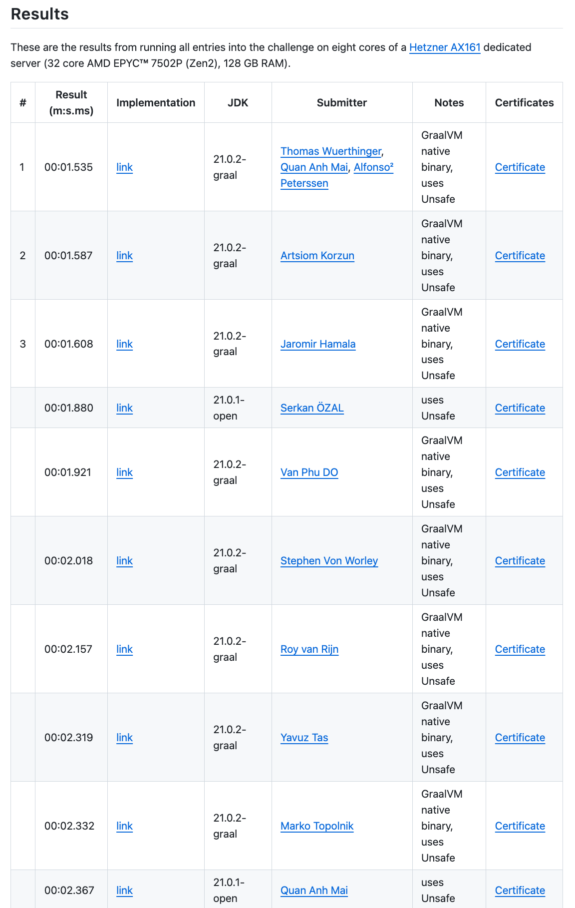
with the results from the 10,000 weather stations

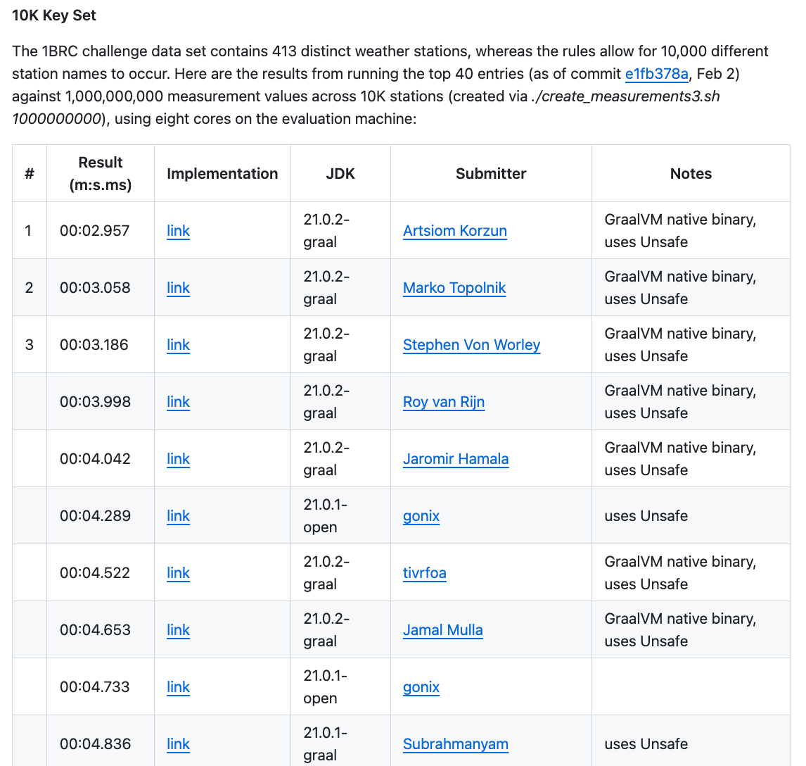
we can see that the #1 solution for 413 stations is no longer in the top 10 for 10,000 stations (although it is #11) and solution #9 has now become the #2. There is quite a bit more fluctuation here. For example, solution #4 with just under 4 seconds for 413 weather stations takes almost 9 seconds for 10,000 weather stations

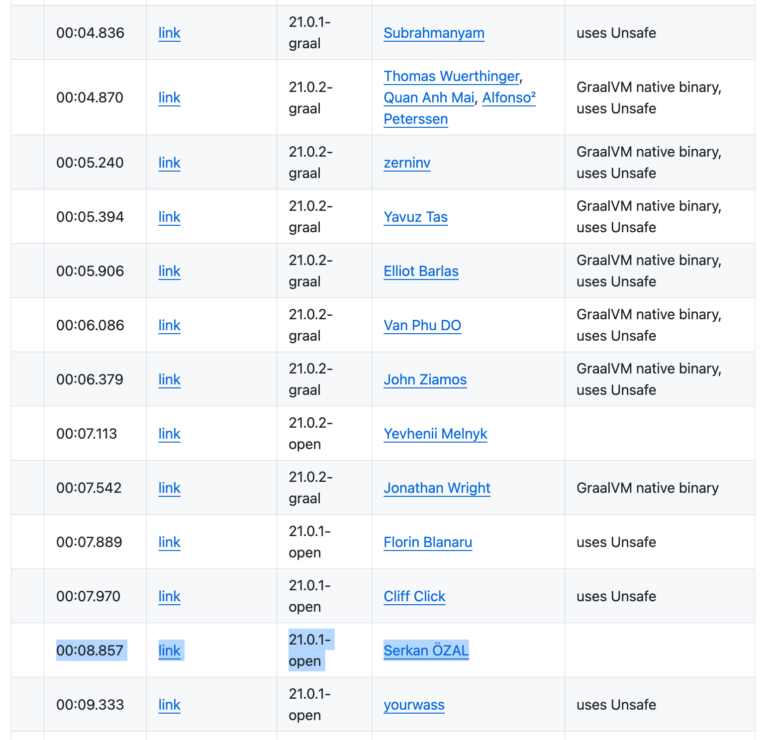
This is not too surprising, given that these implementation were very much tailored for the data at hand (the 413 stations) but, data doesn’t always stay the same – actually it rarely does. This is another big advantage of SQL: it’s declarative. So, instead of having to tweak your code, you can run the exact same query and rely on the SQL engine to do what it does best: getting you accurate results as fast as possible.

Generating the file

The file containing 10,000 weather stations can be generated with a new create_measurements3.sh file. The size of the new file is different than before. The additional repeated station names add about 3 additional GB:

$ ls -alh measurements_*
-rw-r--r--. 1 oracle oinstall 16G Feb 28 16:56 measurements_10k.txt
-rw-r--r--. 1 oracle oinstall 13G Feb 28 17:04 measurements_413.txt

Running the query

10,000 weather stations will make the returned string rather long, too long to be returned as a VARCHAR2 data type. Hence, the following tests will use the “SQL-style” way of aggregating and returning 413 and 10,000 rows, and not concatenating them into one long string. We have already proven earlier on that the string concatenation doesn’t add much additional overhead to the overall query execution, so not creating the string will not severely impact our results.

Returning 413 rows

SQL> SELECT /*+ PARALLEL(128) */
       station_name,
       MIN(measurement) AS min_measurement,
       ROUND(AVG(measurement), 1) AS mean_measurement,
       MAX(measurement) AS max_measurement
 FROM EXTERNAL
 (
   (
     station_name  VARCHAR2(100),
     measurement   NUMBER(3,1)
   )
   TYPE oracle_loader
   DEFAULT DIRECTORY brc
   ACCESS PARAMETERS
   (
     RECORDS DELIMITED BY NEWLINE
     IO_OPTIONS (NODIRECTIO)
     FIELDS TERMINATED BY ';'
     (
       station_name CHAR(100),
       measurement  CHAR(5)
     )
   )
   LOCATION ('measurements_413.txt')
   REJECT LIMIT UNLIMITED
 )
 GROUP BY station_name
 ORDER BY station_name;

STATION_NAME		   MIN_MEASUREMENT MEAN_MEASUREMENT MAX_MEASUREMENT
-------------------------- --------------- ---------------- ---------------
Abha				     -29.6		 18	       68.1
Abidjan 			     -26.2		 26	       73.5
Abéché                               -21.9             29.4            80.8
Accra				     -24.2	       26.4	       73.8
Addis Ababa			     -36.6		 16	       64.2
Adelaide			     -31.2	       17.3	       63.4
Aden				     -19.1	       29.1		 76
Ahvaz				     -22.1	       25.4	       74.4
Albuquerque			     -36.2		 14	       65.5
Alexandra			     -38.3		 11	       60.3
Alexandria			     -28.4		 20		 70
...
...
...
Yinchuan				 -38.9		      9 	   58.7
Zagreb					 -37.6		   10.7 	   64.1
Zanzibar City				 -23.3		     26 	   81.5
Zürich                                   -37.8              9.3            60.4
Ürümqi                                   -40.7              7.4            57.6
İzmir                                    -32.8             17.9              70

413 rows selected.

Elapsed: 00:00:03.71

The result is not much different than before, instead of 3.66 seconds, the query takes 3.71 seconds to return. Note, that the main query has also gotten really simple now, it’s just a common GROUP BY aggregation. Next, let’s see the same results with 10,000 stations.

Returning 10,000 rows

SQL> SELECT /*+ PARALLEL(128) */
       station_name,
       MIN(measurement) AS min_measurement,
       ROUND(AVG(measurement), 1) AS mean_measurement,
       MAX(measurement) AS max_measurement
 FROM EXTERNAL
 (
   (
     station_name  VARCHAR2(100),
     measurement   NUMBER(3,1)
   )
   TYPE oracle_loader
   DEFAULT DIRECTORY brc
   ACCESS PARAMETERS
   (
     RECORDS DELIMITED BY NEWLINE
     IO_OPTIONS (NODIRECTIO)
     FIELDS TERMINATED BY ';'
     (
       station_name CHAR(100),
       measurement  CHAR(5)
     )
   )
   LOCATION ('measurements_10k.txt')
   REJECT LIMIT UNLIMITED
 )
 GROUP BY station_name
 ORDER BY station_name;

STATION_NAME		       MIN_MEASUREMENT MEAN_MEASUREMENT MAX_MEASUREMENT
------------------------------ --------------- ---------------- ---------------
-					 -23.8		   10.8 	   38.4
--la					 -16.7		     17 	   51.9
-Amu					   -13		   14.6 	   45.5
-Arc					 -18.9		   14.9 	   44.7
...
...
...
’s B                                     -22.8             10.2            39.1
’sa                                      -14.9             14.9            45.3
’ye                                      -11.4             18.2              47
’ēBe                                     -11.5             19.5            49.3
’īt                                      -15.6               15            46.4
’ŏn                                      -18.7             11.6            41.7

10000 rows selected.

Elapsed: 00:00:04.61

The weather stations do look quite a bit strange and, at first, one would think that the data may be corrupted. But I assure you, that’s the data that’s in the file (probably auto-generated character sequences). To verify, a grep confirms that weather station “’ēBe” (third-last row) is in the file:

$ grep -c "’ēBe" measurements_10k.txt
99586

So the results look legit, and we can see that the query returned 10,000 rows, one per weather station. The important part here is that the very same query took only 4.61 seconds to produce the results compared to the 3.71 seconds before, just 900 milliseconds longer. However, that’s not quite fair just yet. After all, the database is sending 10,000 rows from the server to the client and the client has to iterate over and print these rows. Although in this case, the client is on the server itself, so no network traffic is in the picture, an easy verification of how much overhead sending and printing all these rows adds to the overall query execution is by wrapping the original query with a SELECT COUNT(*). This way, only one row will be returned to the client (and yes, a few more CPU cycles are burned on the server side for the counting):

SQL> SELECT /*+ PARALLEL(128) */ COUNT(*)
FROM
(SELECT
       station_name,
       MIN(measurement) AS min_measurement,
       ROUND(AVG(measurement), 1) AS mean_measurement,
       MAX(measurement) AS max_measurement
 FROM EXTERNAL
 (
   (
     station_name  VARCHAR2(100),
     measurement   NUMBER(3,1)
   )
   TYPE oracle_loader
   DEFAULT DIRECTORY brc
   ACCESS PARAMETERS
   (
     RECORDS DELIMITED BY NEWLINE
     IO_OPTIONS (NODIRECTIO)
     FIELDS TERMINATED BY ';'
     (
       station_name CHAR(100),
       measurement  CHAR(5)
     )
   )
   LOCATION ('measurements_10k.txt')
   REJECT LIMIT UNLIMITED
 )
 GROUP BY station_name
 ORDER BY station_name
);

  COUNT(*)
----------
     10000

Elapsed: 00:00:04.55

As we can see, producing 10,000 rows is not that much additional overhead, about 0.06 seconds from 4.55 seconds to 4.61 seconds.

But the test has shown something more important. Whether it’s 400 or 10,000 weather stations, SQL can deal with it. No rewrite of the statement is required, and the query didn’t get significantly slower either.

Results

Method	Result
External file, `ORACLE_LOADER`, `NODIRECTIO`, 32 cores	6.82s
External file, `ORACLE_LOADER`, `NODIRECTIO`, 64 cores	3.86s
External file, `ORACLE_LOADER`, `NODIRECTIO`, 128 cores	3.66s
External file, `ORACLE_BIGDATA`, 32 cores	8.12s
External file, `ORACLE_BIGDATA`, 64 cores	4.61s
External file, `ORACLE_BIGDATA`, 128 cores	4.05s
Internal table, 32 cores	4.02s
Internal table, 64 cores	2.28s
Internal table, 128 cores	1.85s
Pre-aggregated materialized view, `QUERY_REWRITE_ENABLED=true`	0.03s
External file, 10000 weather stations, `ORACLE_LOADER,` `NODIRECTIO`, 128 cores	4.61s

What’s next?

Well, this challenge has certainly been fun from an educational point of view. Who knew that the ORACLE_BIGDATA Access Driver does so well in parallelizing and reading from CSV files (and probably many others)! And, as shown, Oracle Database can definitely hold its ground when querying and aggregating data, regardless of whether that data is outside or inside Oracle Database.

Of course, there are numerous additional features that Oracle Database provides that could be used to further decrease the query duration. Do you know of any? Perhaps you should try them for yourself and document your findings, too!

25 thoughts on “1 billion row challenge in SQL and Oracle Database”

Richard Sylvester
2024-02-01 at 20:17

Great article, Gerald.

Reply
raajeshwaran
2024-02-02 at 00:00

any reason why Database In-memory was not considered as an option here ?
things would have been different with DBIM in place.

https://github.com/gunnarmorling/1brc?tab=readme-ov-file#32-cores–64-threads

latest fastest implementation in Java, clocks this at 0.32 seconds. Which is like an order of magnitude faster then the Oracle database.

Reply
1. Gerald
  2024-02-02 at 06:58
  
  Definitely worth a try!
  
  Regarding the Java performance, I already stated:
  
  Although I do not care so much about how fast Oracle Database can process the data compared to the Java implementations. Naturally, with Java one can tailor a program for the exact challenge, leveraging SIMD APIs, bit shifting and all the good stuff that will give you the best possible performance without caring about being a multi-user, general-purpose, ACID compliant system. So there is definitely some overhead that can be saved when writing the Java program.
  
  Besides, all of the fastest implementation use Unsafe operations that have all sorts of side effects would there be more running than just this one calculation. With Oracle, there is no Unsafe, so side effects.
  
  Reply
raajeshwaran
2024-02-02 at 00:11

Also It is worth considering the option of having materialized view in place for those aggregation’s with query rewrite enable

Reply
1. Gerald
  2024-02-02 at 06:50
  
  Indeed, worth a try!
  
  Reply
  1. Gerald
    2024-02-05 at 11:12
    
    Hi raajeshwaran,
    
    I have now added “Bonus #5” to show the benefits of Materialized Views and Query Rewrite.
    
    Thanks,
    
    Reply
Amin Adatia
2024-02-02 at 05:02

Excellent !! Thank you

Reply
aminaa49ed2e27e
2024-02-02 at 05:31

Wonder if using in-memory would make a difference

Reply
1. Gerald
  2024-02-02 at 06:50
  
  Most likely, worth a try!
  
  Reply
2. Christoph Lutz
  2024-02-02 at 13:59
  
  In-Memory does make a difference. I was curious and carried out a test with the IM base level feature and an IM column store size of 16G. This brings query response time into the range of ~0.4 sec (Oracle 19.20 on an X9 Exadata). Not quite as fast as the best Java implementations, but in the same ballpark.
  
  Reply
gasparyyc
2024-02-02 at 21:38

Another interesting perspective to highlight (not part of the original challenge) is that those Java implementations are 400+ lines of very advanced code given the optimization level required!
The implementation here is < 30 lines of plain good ol’ SQL with Oracle using External table features.
My point is that based on the number of lines of SQL in Oracle DB, this is the most productive solution!
Excellent article!

Reply
Pingback: One Billion Rows – Gerald’s Challenge – Learning is not a spectator sport
Carl
2024-02-04 at 07:45

Very cool writeup, thanks. If I was Oracle I would be using this article as my sales pitch!

Reply
emmanuelH
2024-02-05 at 02:01

This SQL implementations is much more robust and maintainable than with “modern languages”. I like that. One question: why did’t you run the query from measurements table in BONUS 4 section ?

Reply
1. Gerald
  2024-02-05 at 08:58
  
  Hi emmanuelH,
  
  The IO_OPTIONS (NODIRECTIO) parameter is an ORACLE_LOADER only option. It does not have any impact on the internal measurements table, only when reading from files, hence there was no point rerunning the query on the internal table.
  
  Reply
Alexander Kornbrust
2024-02-05 at 12:45

Gerald,
Thank you for this interesting article. You could optimize the table design by using pctused/pctfree.

In the current design of the benchmark, there is no need to leave 20% free space in a database block.

Less blocks should result in a higher speed

Regards,
Alexander

Reply
1. Gerald
  2024-02-14 at 16:05
  
  Hi Alexander,
  
  Yes, that is a good point, although I doubt that it will make a significant difference as the data is served entirely out of memory.
  
  Thanks,
  
  Reply
raajeshwaran
2024-02-05 at 18:26
Thanks for adding bonus#5 to this blog post.
However i was playing with my local 21c instance using MV and icing on that with Database In-memory. results were Impressive (consistent improvements in logical IO and elapsed timing)
MV
SELECT station_name,
MIN(measurements) AS min_measurement,
ROUND(AVG(measurements), 1) AS mean_measurement,
MAX(measurements) AS max_measurement
FROM demo_test
GROUP BY station_name

call count cpu elapsed disk query current rows

Parse 1 0.00 0.02 0 0 5 0
Execute 1 0.00 0.00 0 0 0 0
Fetch 277 0.00 0.01 0 623 0 41343

total 279 0.00 0.03 0 623 5 41343

Misses in library cache during parse: 1
Optimizer mode: ALL_ROWS
Parsing user id: 164
Number of plan statistics captured: 1

Rows (1st) Rows (avg) Rows (max) Row Source Operation
```
 41343      41343      41343  MAT_VIEW REWRITE ACCESS FULL DEMO_TEST_MV (cr=623 pr=0 pw=0 time=6961 us starts=1 cost=100 size=1860435 card=41343)
```
Database In-memory
SELECT station_name,
MIN(measurements) AS min_measurement,
ROUND(AVG(measurements), 1) AS mean_measurement,
MAX(measurements) AS max_measurement
FROM demo_test
GROUP BY station_name

call count cpu elapsed disk query current rows

Parse 2 0.00 0.00 0 0 0 0
Execute 2 0.00 0.00 0 0 0 0
Fetch 554 0.02 0.03 0 8 0 82686

total 558 0.02 0.03 0 8 0 82686

Misses in library cache during parse: 0
Optimizer mode: ALL_ROWS
Parsing user id: 164
Number of plan statistics captured: 1

Rows (1st) Rows (avg) Rows (max) Row Source Operation
```
 41343      41343      41343  MAT_VIEW REWRITE ACCESS INMEMORY FULL DEMO_TEST_MV (cr=4 pr=0 pw=0 time=5957 us starts=1 cost=5 size=1860435 card=41343)
```
do you think, it is worth to consider “Exadata Smart Flash cache” for this benchmarking results ?

Reply
1. Gerald
  2024-02-06 at 08:47
  
  There are many features that would further improve this query, including Exadata features, yes.
  
  Reply
addidici
2024-02-25 at 08:30

Hi Gerald

My ./mvnw verify fails with JAVA 21 not supported
Using Oracle Linux
What distro and java did you use?

Or is the 1bn row data file available to download from somewhere?

Adrian

Reply
1. Gerald
  2024-02-26 at 08:31
  
  Hi Adrian,
  
  I used OpenJDK 21:
  
  yum install openjdk@21
  
  Thanks,
  
  Reply
addidici
2024-03-02 at 03:44

OK. I cant find that in my repositories. I guess its not available on Oracle Linux. Do you happen to know which repo it is in?
Thanks
Adrian

Reply
1. Gerald
  2024-03-02 at 09:41
  
  I’m also running on Oracle Linux, chances are it’s a repo configuration issue. You can just download OpenJDK from here: https://jdk.java.net/21/
  
  Thanks,
  
  Reply
Pingback: The One Billion Row Challenge and Oracle 23c Free – Fear and Loathing 3.0
Pingback: Bulk insert challange on MongoDB vs APIs (Oracle 23ai and FerretDB) – Osman DİNÇ'in Veri Tabanı Bloğu